🧪 Tutorial¶

This notebook demonstrates how to:

Define and configure multi-well plates (Plate objects).
Simulate 3-Axis Motion System movements.
Generate and execute G-code for precise well reading.
Collect and process spectral data from serial dilutions.

🚀 You can run this tutorial on Google Colab:

📦 1. Installing Required Packages¶

Before running the notebook, install the required dependencies.

pip install polarstar

pip install spectrochempy==0.6.9

📌 Why Install This?

SpectroChemPy is used for processing, analyzing, and visualizing spectral data.

Version 0.6.9 ensures compatibility with the provided Jupyter Notebook.

🧪 Plate Setup & visualization¶

This Section demonstrates the setup and visualization of multi-well plates with serial dilutions.

It includes:

Two different plates: A 2x3 plate and an 8x12 plate.
Serial dilution setup for Fluorescein, Rhodamine B, and other substances.
G-code path visualization using the Motion System simulation.

🔧 Import Polarstar Library¶

We import necessary modules for handling different plates and visualization.

from polarstar import Plate, CNCController, load_plate

🛠️ Defining a 2x3 Well Plate¶

The first plate (plate_2x3) consists of 2 rows × 3 columns.

We define its properties such as:

Well spacing (x_spacing = 39, y_spacing = 39 mm)
Z-axis safe height (z_safe = 10)
Offsets for calibration (offset_y = -80, offset_z = -5)

plate_2x3 = Plate(rows=2,
              cols=3,
              x_spacing = 39,
              y_spacing = 39,
              z_read = -5,
              offset_y = -80,
              offset_z = -5,
              diameter = 35,
              z_safe = 10
              )

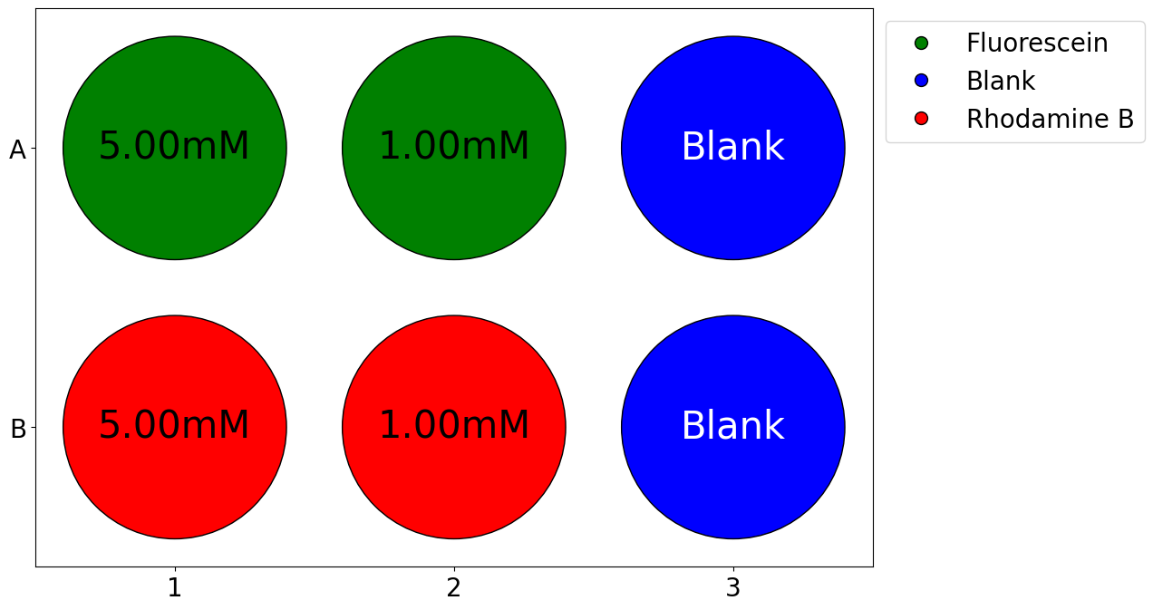
🔬 Serial Dilutions in the 2x3 Plate¶

Fluorescein (green) starts from A1, with a 5x dilution across two wells.
Rhodamine B (red) starts from B1, also with a 5x dilution across two wells.
Blanks (blue) are added at A3 and B3 for control measurements.

# Fill serial dilutions starting from position A1
plate_2x3.set_serial_dilutions(
    start_pos="A1",
    initial_concentration=5,  # 1 mM
    dilution_factor=5,
    num_dilutions=2,
    substance="Fluorescein",
    color="green"
)

# Fill serial dilutions starting from position A1
plate_2x3.set_serial_dilutions(
    start_pos="B1",
    initial_concentration=5,  # 1 mM
    dilution_factor=5,
    num_dilutions=2,
    substance="Rhodamine B",
    color="red"
)

# Add a custom value in position B1
plate_2x3.set_custom(pos="A3", value="Blank", substance="Blank", color="blue")
plate_2x3.set_custom(pos="B3", value="Blank", substance="Blank", color="blue")

📊 Plate Visualization & CNC Simulation¶

A graphical representation of the plate wells is plotted.
The CNC controller simulates the G-code movement.

plate_2x3.plot_plate(well_font_size=30, legend_font_size=20, tick_font_size=20)

# Create a CNC controller object
cnc = CNCController()


# Visualize the plate and G-code path
cnc.simulate(plate_2x3)

🛠️ Defining an 8x12 Well Plate¶

The second plate (plate) is a standard 96-well plate with 8 rows × 12 columns.

Properties include: - Well spacing (x_spacing = 9, y_spacing = 9 mm) - Z-axis safe height (z_safe = 10) - Calibration offsets (offset_y = -90, offset_z = -5)

plate = Plate(rows=8,
              cols=12,
              x_spacing = 9,
              y_spacing = 9,
              z_read = -5,
              offset_y = -90,
              offset_z = -5,
              diameter = 6.94,
              z_safe = 10
              )

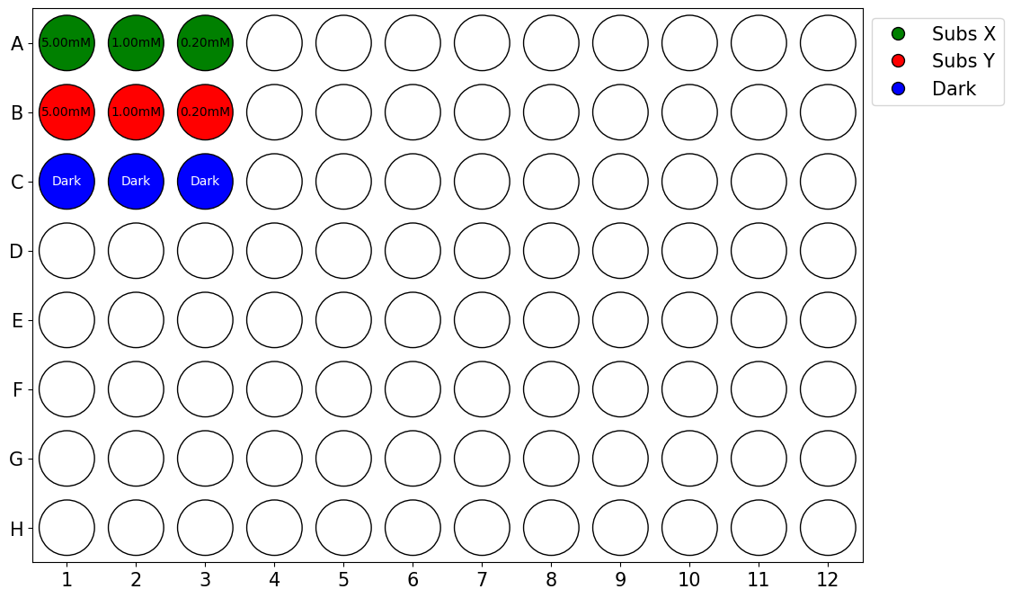
🔬 Serial Dilutions in the 8x12 Plate¶

Substance X (green) starts from A1, with a 5x dilution across three wells.
Substance Y (red) starts from B1, also with a 5x dilution across three wells.
Dark Spectrum (blue) is added to C1, C2, and C3 for baseline measurements.

# Serial dilution for Substance X
plate.set_serial_dilutions(
    start_pos="A1",
    initial_concentration=5,  # 5 mM
    dilution_factor=5,
    num_dilutions=3,
    substance="Subs X",
    color="green"
)

# Serial dilution for Substance Y
plate.set_serial_dilutions(
    start_pos="B1",
    initial_concentration=5,  # 5 mM
    dilution_factor=5,
    num_dilutions=3,
    substance="Subs Y",
    color="red"
)

# Add dark spectrum reference wells
plate.set_custom(pos="C1", value="Dark", substance="Dark", color="blue")
plate.set_custom(pos="C2", value="Dark", substance="Dark", color="blue")
plate.set_custom(pos="C3", value="Dark", substance="Dark", color="blue")

📂 Saving and Loading Plates¶

To save or load a plate’s state from a .star file, use the save() method and the load_plate() function.

This allows reproducible experiments by preserving well data, configurations, and plate parameters.

💾 Saving a Plate’s State

The .star format stores:

Substances and their concentrations in wells.
Custom configurations.
Plate dimensions and offsets for CNC automation.

# Save the plate state to 'my_plate.star'
plate.save('my_plate')

Data successfully saved to my_plate.star

'my_plate.star'

📂 Loading a Saved Plate

Use load_plate() to restore a previously saved plate:

# Load a plate from the file 'my_plate.star'
loaded_plate = load_plate('my_plate.star')

✅ Why Load?

Restores the exact same plate state (wells, concentrations, substances).

Avoids manual setup when continuing experiments.

Useful for batch processing of multiple plates.

📊 Plate Visualization & CNC Simulation¶

The plate layout is plotted, showing well contents.
A CNC controller is created to simulate movement.

loaded_plate.plot_plate(well_font_size=10, legend_font_size=15, tick_font_size=15)

# Create a CNC controller object
cnc = CNCController()


# Visualize the plate and G-code path
cnc.simulate(loaded_plate)

📡 Automated Spectral Data Collection¶

This section simulates spectral data collection using mocked serial communication.

It includes:

CNC command execution,
Spectral data simulation for different well samples,
Data logging in a CSV file for further analysis.

🔧 Import Required Libraries¶

We import necessary modules for handling serial communication, data simulation, and file operations.

import pandas as pd
import numpy as np
import re
import os
from datetime import datetime

📊 Spectral Data Simulation¶

The function get_spectrum_csv() processes well readings from the CNC.

It:

Extracts the well label,
Simulates absorption spectra based on substance type and concentration,
Adds Gaussian noise to simulate real measurements,
Saves the generated data in a CSV file for later analysis.

def get_spectrum_csv(line, csv_filename="spectrum.csv",
                     wavelengths=np.linspace(350, 900, 650, dtype=int),
                     initial_concentration=5.0, dilution_factor=5,
                     initial_intensity=1900, noise_level=0.005, seed=42,
                     dark_spectrum=150):
    """
    Processes a well-reading command, extracts the well label, calculates the corresponding
    absorption spectrum, and saves the data in a CSV file.

    The function determines the concentration of the serial dilution and generates an absorption spectrum
    based on a Gaussian distribution centered at the specific absorption peak of the substance associated
    with the well. The spectrum includes Gaussian noise to simulate real measurements.


    Parameters
    ----------
    line : str
        Command in the format 'Read well at A1', where 'A' can be any letter and '1' can be any number.
    csv_filename : str, optional
        Name of the CSV file where data will be stored (default: "spectrum.csv").
    wavelengths : array-like, optional
        Array of wavelengths in nm (default: 350 to 900 nm with 650 points).
    initial_concentration : float, optional
        Initial solution concentration in mM (default: 5.0 mM).
    dilution_factor : int, optional
        Dilution factor at each step (default: 5).
    initial_intensity : float, optional
        Maximum initial intensity of the spectrum (default: 1900).
    noise_level : float, optional
        Relative noise level (default: 0.005, or 0.5% of the signal intensity).
    seed : int, optional
        Random seed value used for generating Gaussian noise (default: 42).

    Returns
    -------
    None
        The processed data is saved in the specified CSV file.

    Raises
    ------
    ValueError
        If the command is not in the expected format 'Read well at A1'.
    """
    np.random.seed(seed)
    match = re.search(r"([A-Z]\d+)", line)
    if not match:
        raise ValueError("Invalid format. The command must be in the format 'Read well at A1'.")

    well_label = match.group(1)  # Extracts the well label (e.g., A1, B2)
    well_letter = well_label[0]  # Extracts the letter from the label (e.g., "A" or "B")
    well_number = int(re.search(r"\d+", well_label).group())  # Extracts the well number


    # Handle wells with letters other than A and B
    if well_letter not in ['A', 'B']:
        # Create a horizontal line at dark spectrum level
        spectrum = np.full_like(wavelengths, dark_spectrum, dtype=float)
        # Add small noise to make it more realistic
        noise = np.random.normal(0, noise_level * dark_spectrum, size=spectrum.shape)
        spectrum += noise
    else:
        # Define the absorption peak depending on the well label
        peak_wavelengths = {"A": 500, "B": 700}  # Substance X and Y
        peak_wavelength = peak_wavelengths.get(well_letter)

        # Calculate the concentration for that specific well
        concentration = initial_concentration / (dilution_factor ** (well_number - 1))

        # Simulate the absorption spectrum using a Gaussian distribution
        fwhm = 40  # Full width at half maximum of the peak
        sigma = fwhm / (2 * np.sqrt(2 * np.log(2)))  # Convert FWHM to standard deviation

        intensity_factor = initial_intensity * concentration / initial_concentration  # Adjustable scaling factor

        # Generate spectrum and add dark spectrum offset
        spectrum = intensity_factor * np.exp(-((wavelengths - peak_wavelength) ** 2) / (2 * sigma ** 2)) + dark_spectrum

        # Add Gaussian noise to the spectrum
        noise = np.random.normal(0, noise_level * initial_intensity, size=spectrum.shape)
        spectrum += noise  # Add noise to the spectrum

    # Create DataFrame with the data
    data_dict = {
        "Timestamp": datetime.now().strftime("%Y-%m-%d %H:%M:%S"),
        "Label": well_label,
        "Concentration (mM)": concentration if well_letter != 'C' else 0.0
    }
    data_dict.update({w: s for w, s in zip(wavelengths, spectrum)})

    spectrum_df = pd.DataFrame([data_dict])

    # Check if the file exists to determine if the header is needed
    write_header = not os.path.exists(csv_filename)

    # Save data to CSV (append mode)
    spectrum_df.to_csv(csv_filename, mode='a', header=write_header, index=False)

    print(f"Well {well_label} data added to file {csv_filename}")

🎛️ Mocking CNC Serial Communication¶

We simulate CNC communication by:

Mocking the serial port so the CNC always responds with 'ok' and <Idle>,
Ensuring the CNC behaves like it is waiting for commands.

from unittest.mock import MagicMock, patch
import serial
import time
import os

# Mock for the serial port
mock_serial = MagicMock(spec=serial.Serial)

#colocar idle pq o codigo espera que a cnc responda idel quando ela nao esta fazendo nada
# Configure mock behavior
mock_serial.is_open = True  # Simulates that the port is open
mock_serial.readline.side_effect = [
    b'ok\n',  # CNC responses to a command
    b'<Idle>\n',  # 'Idle' state
] * 100  # Repeats to simulate multiple responses

mock_serial.in_waiting = 3  # Simulates bytes available in the buffer

🛠️ Running CNC Controller with a `Plate` Object¶

Now, we:

Patch the serial.Serial object to use our mock.
Instantiate the CNC controller.
Send a Plate object to the CNC for processing.

csv_filename = 'spectrum1.csv'

# Patching to replace 'serial.Serial' with 'mock_serial'
with patch('serial.Serial', return_value=mock_serial):
    # Instantiate the CNC controller
    cnc_controller = CNCController(port='COM1')

    # Register a callback for the 'read' command (retirar)
    cnc_controller.register_callback("read", get_spectrum_csv, csv_filename=csv_filename)

    # Execute G-code sending
    cnc_controller.send_gcode(loaded_plate)

# Display final output
print("Test successfully completed!")

Sent: G21; Set units to millimeters
CNC confirmed 'OK' for: G21; Set units to millimeters
Sent: G90; Use absolute positioning
CNC Response: ok
CNC confirmed 'OK' for: G90; Use absolute positioning
Sent: G0 Z0.00
CNC Response: ok
CNC confirmed 'OK' for: G0 Z0.00
Sent: G0 X0.00 Y-90.00 Z0.00; Move to above well at (0, 0)
CNC Response: ok
CNC confirmed 'OK' for: G0 X0.00 Y-90.00 Z0.00; Move to above well at (0, 0)
Sent: G0 Z5.00; Lower to reading height
CNC Response: ok
CNC confirmed 'OK' for: G0 Z5.00; Lower to reading height
CNC Status: <Idle>
Well A1 data added to file spectrum1.csv
Sent: G0 Z0.00; Raise back to safe height
CNC confirmed 'OK' for: G0 Z0.00; Raise back to safe height
Sent: G0 X9.00 Y-90.00 Z0.00; Move to above well at (0, 1)
CNC Response: ok
CNC confirmed 'OK' for: G0 X9.00 Y-90.00 Z0.00; Move to above well at (0, 1)
Sent: G0 Z5.00; Lower to reading height
CNC Response: ok
CNC confirmed 'OK' for: G0 Z5.00; Lower to reading height
CNC Status: <Idle>
Well A2 data added to file spectrum1.csv
Sent: G0 Z0.00; Raise back to safe height
CNC confirmed 'OK' for: G0 Z0.00; Raise back to safe height
Sent: G0 X18.00 Y-90.00 Z0.00; Move to above well at (0, 2)
CNC Response: ok
CNC confirmed 'OK' for: G0 X18.00 Y-90.00 Z0.00; Move to above well at (0, 2)
Sent: G0 Z5.00; Lower to reading height
CNC Response: ok
CNC confirmed 'OK' for: G0 Z5.00; Lower to reading height
CNC Status: <Idle>
Well A3 data added to file spectrum1.csv
Sent: G0 Z0.00; Raise back to safe height
CNC confirmed 'OK' for: G0 Z0.00; Raise back to safe height
Sent: G0 X0.00 Y-81.00 Z0.00; Move to above well at (1, 0)
CNC Response: ok
CNC confirmed 'OK' for: G0 X0.00 Y-81.00 Z0.00; Move to above well at (1, 0)
Sent: G0 Z5.00; Lower to reading height
CNC Response: ok
CNC confirmed 'OK' for: G0 Z5.00; Lower to reading height
CNC Status: <Idle>
Well B1 data added to file spectrum1.csv
Sent: G0 Z0.00; Raise back to safe height
CNC confirmed 'OK' for: G0 Z0.00; Raise back to safe height
Sent: G0 X9.00 Y-81.00 Z0.00; Move to above well at (1, 1)
CNC Response: ok
CNC confirmed 'OK' for: G0 X9.00 Y-81.00 Z0.00; Move to above well at (1, 1)
Sent: G0 Z5.00; Lower to reading height
CNC Response: ok
CNC confirmed 'OK' for: G0 Z5.00; Lower to reading height
CNC Status: <Idle>
Well B2 data added to file spectrum1.csv
Sent: G0 Z0.00; Raise back to safe height
CNC confirmed 'OK' for: G0 Z0.00; Raise back to safe height
Sent: G0 X18.00 Y-81.00 Z0.00; Move to above well at (1, 2)
CNC Response: ok
CNC confirmed 'OK' for: G0 X18.00 Y-81.00 Z0.00; Move to above well at (1, 2)
Sent: G0 Z5.00; Lower to reading height
CNC Response: ok
CNC confirmed 'OK' for: G0 Z5.00; Lower to reading height
CNC Status: <Idle>
Well B3 data added to file spectrum1.csv
Sent: G0 Z0.00; Raise back to safe height
CNC confirmed 'OK' for: G0 Z0.00; Raise back to safe height
Sent: G0 X0.00 Y-72.00 Z0.00; Move to above well at (2, 0)
CNC Response: ok
CNC confirmed 'OK' for: G0 X0.00 Y-72.00 Z0.00; Move to above well at (2, 0)
Sent: G0 Z5.00; Lower to reading height
CNC Response: ok
CNC confirmed 'OK' for: G0 Z5.00; Lower to reading height
CNC Status: <Idle>
Well C1 data added to file spectrum1.csv
Sent: G0 Z0.00; Raise back to safe height
CNC confirmed 'OK' for: G0 Z0.00; Raise back to safe height
Sent: G0 X9.00 Y-72.00 Z0.00; Move to above well at (2, 1)
CNC Response: ok
CNC confirmed 'OK' for: G0 X9.00 Y-72.00 Z0.00; Move to above well at (2, 1)
Sent: G0 Z5.00; Lower to reading height
CNC Response: ok
CNC confirmed 'OK' for: G0 Z5.00; Lower to reading height
CNC Status: <Idle>
Well C2 data added to file spectrum1.csv
Sent: G0 Z0.00; Raise back to safe height
CNC confirmed 'OK' for: G0 Z0.00; Raise back to safe height
Sent: G0 X18.00 Y-72.00 Z0.00; Move to above well at (2, 2)
CNC Response: ok
CNC confirmed 'OK' for: G0 X18.00 Y-72.00 Z0.00; Move to above well at (2, 2)
Sent: G0 Z5.00; Lower to reading height
CNC Response: ok
CNC confirmed 'OK' for: G0 Z5.00; Lower to reading height
CNC Status: <Idle>
Well C3 data added to file spectrum1.csv
Sent: G0 Z0.00; Raise back to safe height
CNC confirmed 'OK' for: G0 Z0.00; Raise back to safe height
Sent: G0 X0 Y0; Return
CNC Response: ok
CNC confirmed 'OK' for: G0 X0 Y0; Return
Sent: G0 Z0; Return
CNC Response: ok
CNC confirmed 'OK' for: G0 Z0; Return
Sent: M30; End of program
CNC Response: ok
CNC confirmed 'OK' for: M30; End of program
CNC connection closed.
Test successfully completed!

📜 Using a G-code String¶

Instead of using the Plate object directly, we:

Generate G-code as a string.
Send it to the CNC instead of dynamically generating it.

gcode = loaded_plate.generate_gcode()

csv_filename = 'spectrum2.csv'

# Patching to replace 'serial.Serial' with 'mock_serial'
with patch('serial.Serial', return_value=mock_serial):
    # Instantiate the CNC controller
    cnc_controller = CNCController(port='COM1')

    # Register a callback for the 'read' command (retirar)
    cnc_controller.register_callback("read", get_spectrum_csv, csv_filename=csv_filename)

    # Execute G-code sending
    cnc_controller.send_gcode(gcode)

# Display final output
print("Test successfully completed!")

Sent: G21; Set units to millimeters
CNC Response: ok
CNC confirmed 'OK' for: G21; Set units to millimeters
Sent: G90; Use absolute positioning
CNC Response: ok
CNC confirmed 'OK' for: G90; Use absolute positioning
Sent: G0 Z0.00
CNC Response: ok
CNC confirmed 'OK' for: G0 Z0.00
Sent: G0 X0.00 Y-90.00 Z0.00; Move to above well at (0, 0)
CNC Response: ok
CNC confirmed 'OK' for: G0 X0.00 Y-90.00 Z0.00; Move to above well at (0, 0)
Sent: G0 Z5.00; Lower to reading height
CNC Response: ok
CNC confirmed 'OK' for: G0 Z5.00; Lower to reading height
CNC Status: <Idle>
Well A1 data added to file spectrum2.csv
Sent: G0 Z0.00; Raise back to safe height
CNC confirmed 'OK' for: G0 Z0.00; Raise back to safe height
Sent: G0 X9.00 Y-90.00 Z0.00; Move to above well at (0, 1)
CNC Response: ok
CNC confirmed 'OK' for: G0 X9.00 Y-90.00 Z0.00; Move to above well at (0, 1)
Sent: G0 Z5.00; Lower to reading height
CNC Response: ok
CNC confirmed 'OK' for: G0 Z5.00; Lower to reading height
CNC Status: <Idle>
Well A2 data added to file spectrum2.csv
Sent: G0 Z0.00; Raise back to safe height
CNC confirmed 'OK' for: G0 Z0.00; Raise back to safe height
Sent: G0 X18.00 Y-90.00 Z0.00; Move to above well at (0, 2)
CNC Response: ok
CNC confirmed 'OK' for: G0 X18.00 Y-90.00 Z0.00; Move to above well at (0, 2)
Sent: G0 Z5.00; Lower to reading height
CNC Response: ok
CNC confirmed 'OK' for: G0 Z5.00; Lower to reading height
CNC Status: <Idle>
Well A3 data added to file spectrum2.csv
Sent: G0 Z0.00; Raise back to safe height
CNC confirmed 'OK' for: G0 Z0.00; Raise back to safe height
Sent: G0 X0.00 Y-81.00 Z0.00; Move to above well at (1, 0)
CNC Response: ok
CNC confirmed 'OK' for: G0 X0.00 Y-81.00 Z0.00; Move to above well at (1, 0)
Sent: G0 Z5.00; Lower to reading height
CNC Response: ok
CNC confirmed 'OK' for: G0 Z5.00; Lower to reading height
CNC Status: <Idle>
Well B1 data added to file spectrum2.csv
Sent: G0 Z0.00; Raise back to safe height
CNC confirmed 'OK' for: G0 Z0.00; Raise back to safe height
Sent: G0 X9.00 Y-81.00 Z0.00; Move to above well at (1, 1)
CNC Response: ok
CNC confirmed 'OK' for: G0 X9.00 Y-81.00 Z0.00; Move to above well at (1, 1)
Sent: G0 Z5.00; Lower to reading height
CNC Response: ok
CNC confirmed 'OK' for: G0 Z5.00; Lower to reading height
CNC Status: <Idle>
Well B2 data added to file spectrum2.csv
Sent: G0 Z0.00; Raise back to safe height
CNC confirmed 'OK' for: G0 Z0.00; Raise back to safe height
Sent: G0 X18.00 Y-81.00 Z0.00; Move to above well at (1, 2)
CNC Response: ok
CNC confirmed 'OK' for: G0 X18.00 Y-81.00 Z0.00; Move to above well at (1, 2)
Sent: G0 Z5.00; Lower to reading height
CNC Response: ok
CNC confirmed 'OK' for: G0 Z5.00; Lower to reading height
CNC Status: <Idle>
Well B3 data added to file spectrum2.csv
Sent: G0 Z0.00; Raise back to safe height
CNC confirmed 'OK' for: G0 Z0.00; Raise back to safe height
Sent: G0 X0.00 Y-72.00 Z0.00; Move to above well at (2, 0)
CNC Response: ok
CNC confirmed 'OK' for: G0 X0.00 Y-72.00 Z0.00; Move to above well at (2, 0)
Sent: G0 Z5.00; Lower to reading height
CNC Response: ok
CNC confirmed 'OK' for: G0 Z5.00; Lower to reading height
CNC Status: <Idle>
Well C1 data added to file spectrum2.csv
Sent: G0 Z0.00; Raise back to safe height
CNC confirmed 'OK' for: G0 Z0.00; Raise back to safe height
Sent: G0 X9.00 Y-72.00 Z0.00; Move to above well at (2, 1)
CNC Response: ok
CNC confirmed 'OK' for: G0 X9.00 Y-72.00 Z0.00; Move to above well at (2, 1)
Sent: G0 Z5.00; Lower to reading height
CNC Response: ok
CNC confirmed 'OK' for: G0 Z5.00; Lower to reading height
CNC Status: <Idle>
Well C2 data added to file spectrum2.csv
Sent: G0 Z0.00; Raise back to safe height
CNC confirmed 'OK' for: G0 Z0.00; Raise back to safe height
Sent: G0 X18.00 Y-72.00 Z0.00; Move to above well at (2, 2)
CNC Response: ok
CNC confirmed 'OK' for: G0 X18.00 Y-72.00 Z0.00; Move to above well at (2, 2)
Sent: G0 Z5.00; Lower to reading height
CNC Response: ok
CNC confirmed 'OK' for: G0 Z5.00; Lower to reading height
CNC Status: <Idle>
Well C3 data added to file spectrum2.csv
Sent: G0 Z0.00; Raise back to safe height
CNC confirmed 'OK' for: G0 Z0.00; Raise back to safe height
Sent: G0 X0 Y0; Return
CNC Response: ok
CNC confirmed 'OK' for: G0 X0 Y0; Return
Sent: G0 Z0; Return
CNC Response: ok
CNC confirmed 'OK' for: G0 Z0; Return
Sent: M30; End of program
CNC Response: ok
CNC confirmed 'OK' for: M30; End of program
CNC connection closed.
Test successfully completed!

📂 Using a G-code File¶

We now:

Load the G-code from a saved file.
Send it to the CNC directly.

# Generate G-code from the plate and save it to a file
gcode = loaded_plate.generate_gcode(
   filename="plate.gcode"  # Output G-code file
)

csv_filename = 'spectrum3.csv'

# Patching to replace 'serial.Serial' with 'mock_serial'
with patch('serial.Serial', return_value=mock_serial):
    # Instantiate the CNC controller
    cnc_controller = CNCController(port='COM1')

    # Register a callback for the 'read' command (retirar)
    cnc_controller.register_callback("read", get_spectrum_csv, csv_filename=csv_filename)

    # Execute G-code sending
    cnc_controller.send_gcode("plate.gcode")

# Display final output
print("Test successfully completed!")

Sent: G21; Set units to millimeters
CNC Response: ok
CNC confirmed 'OK' for: G21; Set units to millimeters
Sent: G90; Use absolute positioning
CNC Response: ok
CNC confirmed 'OK' for: G90; Use absolute positioning
Sent: G0 Z0.00
CNC Response: ok
CNC confirmed 'OK' for: G0 Z0.00
Sent: G0 X0.00 Y-90.00 Z0.00; Move to above well at (0, 0)
CNC Response: ok
CNC confirmed 'OK' for: G0 X0.00 Y-90.00 Z0.00; Move to above well at (0, 0)
Sent: G0 Z5.00; Lower to reading height
CNC Response: ok
CNC confirmed 'OK' for: G0 Z5.00; Lower to reading height
CNC Status: <Idle>
Well A1 data added to file spectrum3.csv
Sent: G0 Z0.00; Raise back to safe height
CNC confirmed 'OK' for: G0 Z0.00; Raise back to safe height
Sent: G0 X9.00 Y-90.00 Z0.00; Move to above well at (0, 1)
CNC Response: ok
CNC confirmed 'OK' for: G0 X9.00 Y-90.00 Z0.00; Move to above well at (0, 1)
Sent: G0 Z5.00; Lower to reading height
CNC Response: ok
CNC confirmed 'OK' for: G0 Z5.00; Lower to reading height
CNC Status: <Idle>
Well A2 data added to file spectrum3.csv
Sent: G0 Z0.00; Raise back to safe height
CNC confirmed 'OK' for: G0 Z0.00; Raise back to safe height
Sent: G0 X18.00 Y-90.00 Z0.00; Move to above well at (0, 2)
CNC Response: ok
CNC confirmed 'OK' for: G0 X18.00 Y-90.00 Z0.00; Move to above well at (0, 2)
Sent: G0 Z5.00; Lower to reading height
CNC Response: ok
CNC confirmed 'OK' for: G0 Z5.00; Lower to reading height
CNC Status: <Idle>
Well A3 data added to file spectrum3.csv
Sent: G0 Z0.00; Raise back to safe height
CNC confirmed 'OK' for: G0 Z0.00; Raise back to safe height
Sent: G0 X0.00 Y-81.00 Z0.00; Move to above well at (1, 0)
CNC Response: ok
CNC confirmed 'OK' for: G0 X0.00 Y-81.00 Z0.00; Move to above well at (1, 0)
Sent: G0 Z5.00; Lower to reading height
CNC Response: ok
CNC confirmed 'OK' for: G0 Z5.00; Lower to reading height
CNC Status: <Idle>
Well B1 data added to file spectrum3.csv
Sent: G0 Z0.00; Raise back to safe height
CNC confirmed 'OK' for: G0 Z0.00; Raise back to safe height
Sent: G0 X9.00 Y-81.00 Z0.00; Move to above well at (1, 1)
CNC Response: ok
CNC confirmed 'OK' for: G0 X9.00 Y-81.00 Z0.00; Move to above well at (1, 1)
Sent: G0 Z5.00; Lower to reading height
CNC Response: ok
CNC confirmed 'OK' for: G0 Z5.00; Lower to reading height
CNC Status: <Idle>
Well B2 data added to file spectrum3.csv
Sent: G0 Z0.00; Raise back to safe height
CNC confirmed 'OK' for: G0 Z0.00; Raise back to safe height
Sent: G0 X18.00 Y-81.00 Z0.00; Move to above well at (1, 2)
CNC Response: ok
CNC confirmed 'OK' for: G0 X18.00 Y-81.00 Z0.00; Move to above well at (1, 2)
Sent: G0 Z5.00; Lower to reading height
CNC Response: ok
CNC confirmed 'OK' for: G0 Z5.00; Lower to reading height
CNC Status: <Idle>
Well B3 data added to file spectrum3.csv
Sent: G0 Z0.00; Raise back to safe height
CNC confirmed 'OK' for: G0 Z0.00; Raise back to safe height
Sent: G0 X0.00 Y-72.00 Z0.00; Move to above well at (2, 0)
CNC Response: ok
CNC confirmed 'OK' for: G0 X0.00 Y-72.00 Z0.00; Move to above well at (2, 0)
Sent: G0 Z5.00; Lower to reading height
CNC Response: ok
CNC confirmed 'OK' for: G0 Z5.00; Lower to reading height
CNC Status: <Idle>
Well C1 data added to file spectrum3.csv
Sent: G0 Z0.00; Raise back to safe height
CNC confirmed 'OK' for: G0 Z0.00; Raise back to safe height
Sent: G0 X9.00 Y-72.00 Z0.00; Move to above well at (2, 1)
CNC Response: ok
CNC confirmed 'OK' for: G0 X9.00 Y-72.00 Z0.00; Move to above well at (2, 1)
Sent: G0 Z5.00; Lower to reading height
CNC Response: ok
CNC confirmed 'OK' for: G0 Z5.00; Lower to reading height
CNC Status: <Idle>
Well C2 data added to file spectrum3.csv
Sent: G0 Z0.00; Raise back to safe height
CNC confirmed 'OK' for: G0 Z0.00; Raise back to safe height
Sent: G0 X18.00 Y-72.00 Z0.00; Move to above well at (2, 2)
CNC Response: ok
CNC confirmed 'OK' for: G0 X18.00 Y-72.00 Z0.00; Move to above well at (2, 2)
Sent: G0 Z5.00; Lower to reading height
CNC Response: ok
CNC confirmed 'OK' for: G0 Z5.00; Lower to reading height
CNC Status: <Idle>
Well C3 data added to file spectrum3.csv
Sent: G0 Z0.00; Raise back to safe height
CNC confirmed 'OK' for: G0 Z0.00; Raise back to safe height
Sent: G0 X0 Y0; Return
CNC Response: ok
CNC confirmed 'OK' for: G0 X0 Y0; Return
Sent: G0 Z0; Return
CNC Response: ok
CNC confirmed 'OK' for: G0 Z0; Return
Sent: M30; End of program
CNC Response: ok
CNC confirmed 'OK' for: M30; End of program
CNC connection closed.
Test successfully completed!

🔬 Spectral Data Analysis: Processing and Plotting¶

This section demonstrates:

Loading spectral data and processing it for analysis.
Visualizing spectra using custom configurations.
Normalizing data, filtering noise, and finding peaks in spectral regions.
Analyzing substance X and Substance Y data for peak detection.

We will use the spectrochempy library for handling spectral data.

⚠️ Recommended Best Practice: Separate Notebooks for Spectral Analysis and Plate Preparation & CNC Execution

While this tutorial integrates the PolarStar library with SpectroChemPy,

it is strongly recommended to perform:

Plate Preparation & CNC Execution with PolarStar in one notebook.
Spectral data analysis with SpectroChemPy in a separate notebook.

📌 Why?

SpectroChemPy modifies Matplotlib styles, which can cause inconsistent plots when used alongside PolarStar.
Isolating both processes prevents style conflicts and ensures clearer debugging and reproducibility.

🔧 Import Required Libraries¶

We import necessary modules for:

Spectral data processing, Peak detection, smoothing and visualization

import spectrochempy as scp
import pandas as pd
import numpy as np
import matplotlib.pyplot as plt
from matplotlib.ticker import AutoMinorLocator

%matplotlib inline

🛠️ Configure Plot Settings¶

We define a custom function configure_plot() to apply consistent styling across all plots.

This function configures:

Ticks and spines,
Axis limits and legends.

# Function to configure plots
def configure_plot(ax, labels=None, ylim=None):
    """
    Configure plot parameters for consistent styling.

    Parameters:
    -----------
    ax : matplotlib.axes.Axes
        The Axes object to configure.
    labels : list of str, optional
        List of labels for the legend.
    ylim : tuple, optional
        Y-axis limits as (ymin, ymax).
    """
    # Configure minor ticks
    ax.xaxis.set_minor_locator(AutoMinorLocator(8))
    ax.yaxis.set_minor_locator(AutoMinorLocator(5))

    # Customize tick styles
    ax.tick_params(axis='x', which='major', length=12, width=2, direction='in', color='black', labelsize='large')
    ax.tick_params(axis='x', which='minor', length=5, width=2, direction='in', color='black', labelsize='large')
    ax.tick_params(axis='y', which='major', length=12, width=2, direction='in', color='black', labelsize='large')
    ax.tick_params(axis='y', which='minor', length=5, width=2, direction='in', color='black', labelsize='large')

    # Adjust spine thickness
    for spine in ax.spines.values():
        spine.set_linewidth(2)

    # Remove top and right spines
    ax.spines['top'].set_visible(False)
    ax.spines['right'].set_visible(False)

    # Set Y-axis limits
    if ylim is not None:
        ax.set_ylim(*ylim)

    # Add legend if labels are provided
    if labels:
        ax.legend(labels=labels, frameon=False)

📊 Load and Process Data¶

Here, we load the spectral data from the CSV file, which contains intensity values for various substances. We separate the numeric columns and prepare them for further analysis.

# Load the CSV file
df = pd.read_csv(csv_filename)

💾 Extracting Numeric Columns¶

We extract numeric columns (intensities) from the dataset, and create a dictionary to store data by label.

numeric_columns = df.select_dtypes(include='number')

numeric_columns.insert(0, 'Label', df['Label'])

# Create a dictionary to store data by label
dfs = {}
labels = numeric_columns['Label'].unique()

for label in labels:
    # Filter data by label
    filtered_df = numeric_columns[numeric_columns['Label'] == label]
    data = filtered_df.iloc[:, 2:].to_numpy()  # Extract intensity values (excluding Timestamp and Label)
    dfs[label] = data.flatten()  # Store the data in the dictionary

# Stack arrays stored in the dictionary
nd_data = np.stack(list(dfs.values()), axis=0)  # Stack data into a multidimensional array

🗂️ Create SpectroChemPy Dataset¶

We convert the stacked spectral data into a SpectroChemPy dataset, which allows us to process and visualize the data more effectively.

# Convert to a SpectroChemPy dataset
dataset = scp.NDDataset(nd_data)

dataset

name	NDDataset_5c50e38b
author	julio@DESKTOP-9C6CP48
created	2025-02-11 02:38:02-03:00
DATA
title
values	[[ 148.7 156.2 ... 147.8 156.6] [ 148.7 156.2 ... 147.8 156.6] ... [ 149.9 150.5 ... 149.8 150.5] [ 149.9 150.5 ... 149.8 150.5]]
shape	(y:9, x:551)

Define Coordinates for Spectral Data

subs = labels  # List of labels
c0 = list(range(len(subs)))  # Indices corresponding to spectra

coord = numeric_columns.columns[2:].to_numpy()
coord

coord0 = scp.Coord(
    data=c0, labels=subs, units="absorbance", title="Wells"
)
coord1 = scp.Coord(data=coord, labels=None, units="nm", title="Wavelength")


mydataset = scp.NDDataset(
    nd_data, coordset=[coord0, coord1], title="Intensity", units="absorbance"
)
mydataset.description = "Dataset criado a partir do empilhamento de espectros"
mydataset.name = "96 well"
mydataset.author = "Júlio G. Maranho"

prefs = mydataset.preferences
prefs.figure.figsize = (9, 5)
mydataset

name	96 well
author	Júlio G. Maranho
created	2025-02-11 02:38:02-03:00
description	Dataset criado a partir do empilhamento de espectros
DATA
title	Intensity
values	[[ 148.7 156.2 ... 147.8 156.6] [ 148.7 156.2 ... 147.8 156.6] ... [ 149.9 150.5 ... 149.8 150.5] [ 149.9 150.5 ... 149.8 150.5]] a.u.
shape	(y:9, x:551)
DIMENSION `x`
size	551
title	Wavelength
coordinates	[ 350 351 ... 899 900] nm
DIMENSION `y`
size	9
title	Wells
coordinates	[ 0 1 ... 7 8] a.u.
labels	[ A1 A2 ... C2 C3]

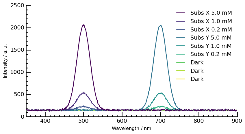
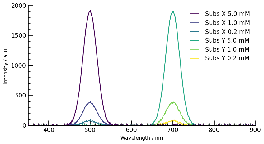
📈 Visualize and Analyze Spectral Data¶

We plot the spectral data for different substances and apply data processing steps, such as:

Subtracting the dark spectrum,
Savitzky-Golay smoothing filter for noise reduction.

labels = [
    'Subs X 5.0 mM',
    'Subs X 1.0 mM',
    'Subs X 0.2 mM',
    'Subs Y 5.0 mM',
    'Subs Y 1.0 mM',
    'Subs Y 0.2 mM',
    'Dark',
    'Dark',
    'Dark'
]

📌Plots the raw spectra with labeled curves for each sample.

ax = mydataset.plot(linewidth=2)
configure_plot(ax, labels=labels, ylim=(0, 2500))

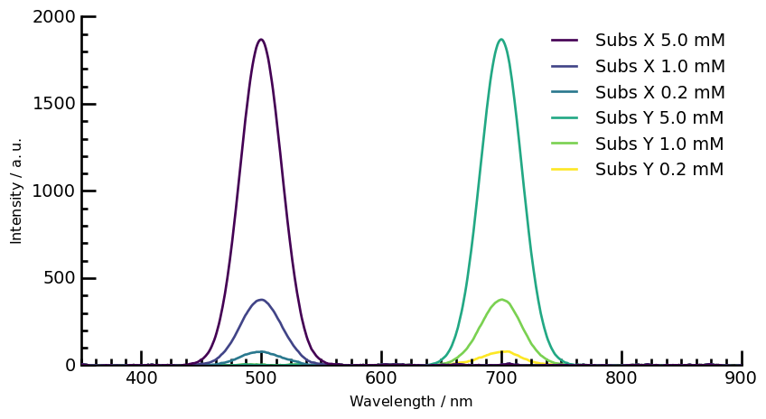
📌Subtract Dark Spectrum (Baseline Correction)

# Subtract the mean Dark spectrum from all other spectra
removed = mydataset[0:6] - mydataset[6:].mean(dim=0)

# Display the resulting dataset
removed

name	96 well
author	Júlio G. Maranho
created	2025-02-11 02:38:02-03:00
description	Dataset criado a partir do empilhamento de espectros
history	2025-02-11 02:38:03-03:00> Slice extracted: (slice(0, 6, None)) 2025-02-11 02:38:03-03:00> Binary operation sub with `96 well` has been performed
DATA
title	Intensity
values	[[ -1.21 5.667 ... -2.021 6.092] [ -1.21 5.667 ... -2.021 6.092] ... [ -1.21 5.667 ... -2.021 6.092] [ -1.21 5.667 ... -2.021 6.092]] a.u.
shape	(y:6, x:551)
DIMENSION `x`
size	551
title	Wavelength
coordinates	[ 350 351 ... 899 900] nm
DIMENSION `y`
size	6
title	Wells
coordinates	[ 0 1 2 3 4 5] a.u.
labels	[ A1 A2 A3 B1 B2 B3]

ax = removed.plot(linewidth=2)
configure_plot(ax, labels=labels, ylim=(0, 2000))

📌 Smooths spectra to reduce noise while preserving peaks.

# Apply Savitzky-Golay filter for smoothing
savgol = removed.savgol_filter(size=11, order=1)

ax = savgol.plot(linewidth=2)
configure_plot(ax, labels=labels, ylim=(0, 2000))

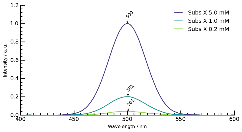
📌 Normalizes the data and detects peaks.

# Split the data into Substance X and Substance Y subsets
X = savgol[:3]
Y = savgol[3:6]

# Normalize Substance X and Substance Y  data
norm_X = X / X.max()
norm_Y = Y / Y.max()

# Find peaks in the normalized data
peakslist_X = [s.find_peaks(prominence=0.01)[0] for s in norm_X]
peakslist_Y = [s.find_peaks(prominence=0.01)[0] for s in norm_Y]

# Select specific regions for Substance X and Substance Y  data
reg_X = norm_X[:, 400.0:600.0]
reg_X.units = "absorbance"
reg_Y = norm_Y[:, 600.0:800.0]
reg_Y.units = "absorbance"

# Set y-axis limits for the plot
ylim = (0, 1.2)

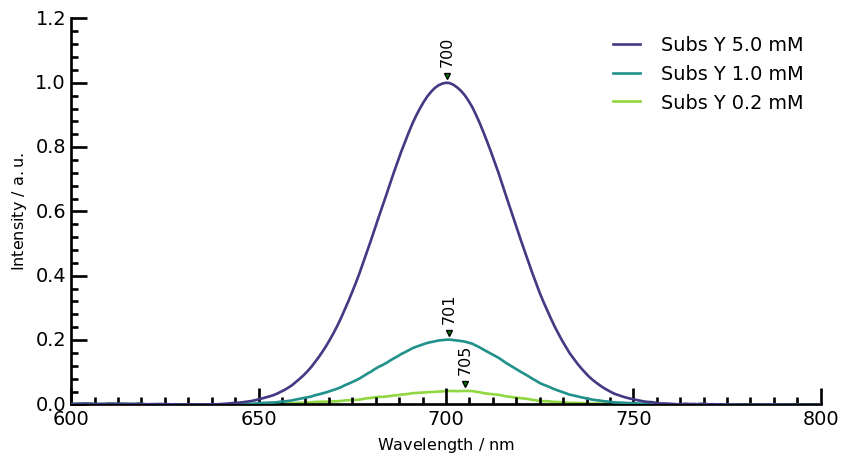
📌 Annotates peaks in the selected spectral regions.

# Plot Sub X spectra with peak annotations
ax = reg_X.plot(linewidth=2)

for peaks in peakslist_X:
    pks = peaks + 0.02
    pks.plot_scatter(
        ax=ax,
        marker="v",
        ms=5,
        color="red",
        clear=False,
        data_only=True,
        ylim=ylim,
    )
    for p in pks:
        x, y = p.x.values, p.values + 0.04
        _ = ax.annotate(
            f"{x.m:0.0f}",
            xy=(x, y),
            xytext=(-5, 0),
            rotation=45,
            textcoords="offset points",
        )

configure_plot(ax, labels=labels[0:3], ylim=ylim)

# Plot Sub Y spectra with peak annotations
ax = reg_Y.plot(linewidth=2)

for peaks in peakslist_Y:
    pks = peaks + 0.02
    pks.plot_scatter(
        ax=ax,
        marker="v",
        ms=5,
        color="red",
        clear=False,
        data_only=True,
        ylim=ylim,
    )
    for p in pks:
        x, y = p.x.values, p.values + 0.04
        _ = ax.annotate(
            f"{x.m:0.0f}",
            xy=(x, y),
            xytext=(-5, 0),
            rotation=90,
            textcoords="offset points",
        )

configure_plot(ax, labels=labels[3:6], ylim=ylim)

🧪 Tutorial¶

📦 1. Installing Required Packages¶

🧪 Plate Setup & visualization¶

🔧 Import Polarstar Library¶

🛠️ Defining a 2x3 Well Plate¶

🔬 Serial Dilutions in the 2x3 Plate¶

📊 Plate Visualization & CNC Simulation¶

🛠️ Defining an 8x12 Well Plate¶

🔬 Serial Dilutions in the 8x12 Plate¶

📂 Saving and Loading Plates¶

📊 Plate Visualization & CNC Simulation¶

📡 Automated Spectral Data Collection¶

🔧 Import Required Libraries¶

📊 Spectral Data Simulation¶

🎛️ Mocking CNC Serial Communication¶

🛠️ Running CNC Controller with a Plate Object¶

📜 Using a G-code String¶

📂 Using a G-code File¶

🔬 Spectral Data Analysis: Processing and Plotting¶

🔧 Import Required Libraries¶

🛠️ Configure Plot Settings¶

📊 Load and Process Data¶

💾 Extracting Numeric Columns¶

🗂️ Create SpectroChemPy Dataset¶

📈 Visualize and Analyze Spectral Data¶

🛠️ Running CNC Controller with a `Plate` Object¶